File:Symmetricwave2.png
From Vigyanwiki

Size of this preview: 800 × 599 pixels. Other resolutions: 320 × 240 pixels | 640 × 479 pixels | 1,024 × 767 pixels | 1,280 × 958 pixels | 1,811 × 1,356 pixels.
Original file (1,811 × 1,356 pixels, file size: 540 KB, MIME type: image/png)
Any autoconfirmed user can overwrite this file from the same source. Please ensure that overwrites comply with the guideline.

|
This physics image could be re-created using vector graphics as an SVG file. This has several advantages; see Commons:Media for cleanup for more information. If an SVG form of this image is available, please upload it and afterwards replace this template with
{{vector version available|new image name}}.
It is recommended to name the SVG file “Symmetricwave2.svg”—then the template Vector version available (or Vva) does not need the new image name parameter. |
Summary
| Description |
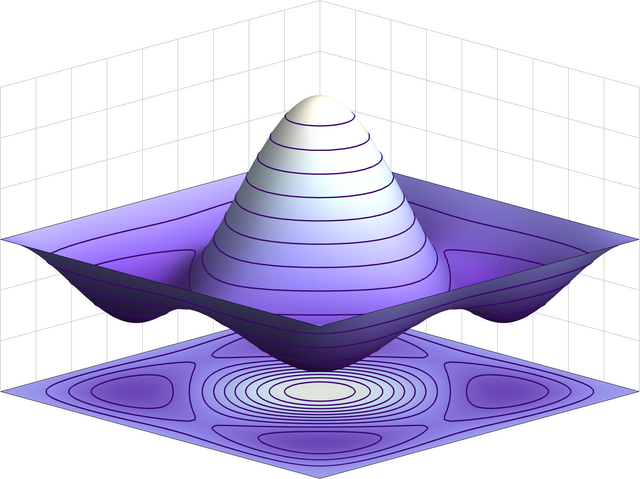
English: Symmetric wavefunction for a (bosonic) 2-particle state in an infinite square well potential. |
| Source | Own work |
| Author | TimothyRias |
Licensing
I, the copyright holder of this work, hereby publish it under the following licence:
This file is licensed under the Creative Commons Attribution 3.0 Unported licence.
- You are free:
- to share – to copy, distribute and transmit the work
- to remix – to adapt the work
- Under the following conditions:
- attribution – You must give appropriate credit, provide a link to the licence, and indicate if changes were made. You may do so in any reasonable manner, but not in any way that suggests the licensor endorses you or your use.
Summary
This 3D graph shows the wavefunction for the 2-particle bosonic state for the one dimensional infinite square well at the same energy as the fermionic 2-particle groundstate. (See for example D.J. Griffiths, Introduction to quantum mechanics, Prentice Hall , 1995, section 5.1.1) The picture was created using Mathematica 6.0 using the following code:
$Assumptions = {n \[Element] Integers, m \[Element] Integers};
f[n_, x_] := Sqrt[2] Sin[n \[Pi] x];
s[n_, m_] :=
 Function[{x, y}, (f[n, x] f[m, y] + f[n, y] f[m, x])/Sqrt[2]];
swave2 = Plot3D[Evaluate[-s[3, 1][x, y]], {x, 0, 1}, {y, 0, 1},
  PlotPoints -> 35,
  PlotRange -> {-2.5, 3.5},
  MeshFunctions -> {#3 &},
  MeshStyle ->
   Directive[ColorData["DeepSeaColors"][.1], Thickness[.002]],
  Mesh -> 10,
  ColorFunction -> "LakeColors",
  BoxRatios -> {1, 1, .7},
  Boxed -> False,
  Axes -> False];
sgroundplot = Plot3D[-3, {x, 0, 1}, {y, 0, 1},
  MeshFunctions -> {s[1, 3][#1, #2] &},
  Mesh -> 10,
  MeshStyle ->
   Directive[ColorData["DeepSeaColors"][.1], Thickness[.002]],
  PlotPoints -> 50,
  ColorFunction -> (ColorData["LakeColors"][(-s[1, 3][#1, #2] + 2.5)/
      6] &)];
swave3 = Show[{swave2, sgroundplot},
 PlotRange -> {{0, 1}, {0, 1}, {-3, 3}},
 Axes -> None,
 PlotRangePadding -> None,
 ImagePadding -> 1,
 FaceGrids -> {
   {{-1, 0, 0}, {Table[i, {i, 0, 1, 1/9}],
     Table[i, {i, -3, 3, 1}]}},
   {{0, -1, 0}, {Table[i, {i, 0, 1, 1/9}], Table[i, {i, -3, 3, 1}]}}
   },
 ViewPoint -> 1000 {5, 5, 2},
 ViewVertical -> {0, 0, 1},
 ViewCenter -> {.5, .5, 0},
 ImageSize -> 600]
Export["Symmetricwave2.png", swave3, "PNG"]
File history
Click on a date/time to view the file as it appeared at that time.
| Date/Time | Thumbnail | Dimensions | User | Comment | |
|---|---|---|---|---|---|
| current | 21:22, 19 February 2024 | | 1,811 × 1,356 (540 KB) | wikimediacommons>Jähmefyysikko | Antialiasing and higher resolution |
File usage
The following page uses this file: